🩻 ✏️ Lessons in Python Ray Tracing
I found this excellent book about implementing a ray tracer in C: raytracing.github.io/books/RayTracingInOneWeekend.html. As you may have discerned from the title, I’ve attempted to implement this ray tracer in Python. Here’s the source code: github.com/a-vinod/ray-tracer2
The astute of you may realize that this is a fool’s errand. The program runtime scales at O(height*width*aa_samples*recursion_depth) so of course this will be slow with Python! But it was still very interesting to see how quickly I hit the limits of a reasonable wait between iterations of generating an image. Also, it was worth learning about ray tracing without the pleasure of debugging seg faults.
As for packages, I’m limiting myself to numpy for math and cv2 for image import/export. I also used some convenience packages that I’ll go into later. Yes this isn’t 🍦 Python there’s some chocolate sauce too.
High-Level Program Flow
ray_tracer2/camera.py
def render(self, world: World) -> np.ndarray:
    ...
        for y in range(self.image_height):
            for x in range(self.image_width):
                ...
                for aa in range(self.aa_samples):
                    ...
                    color += self.ray_color(ray, world, 50)
                colors[y][x] = 255*color/self.aa_samples
This render() function is the top-level nested loop that populates the 2D numpy colors array with the RGB values for each pixel.
The ray_color() function traces the ray originating from the camera to each sampled point in each pixel in the viewport of the world. When the ray hits something in the world, the World::hit(Ray) function returns a HitRecord that has some information about the hit including the material to determine if/how the subsequent ray scatters.
The World::hit(Ray) iterates through the different objects in the world (currently only spheres) and invokes Sphere::hit(Ray) to compute the intersection of the ray and the sphere.
ray_tracer2/hittable.py
    def hit(self, ray: Ray, tmin: float, tmax: float) -> (HitRecord, bool):
        """
        x^2 + y^2 + z^2 = r^2
        (Cx-x)^2 + (Cy-y)^2 + (Cz-z)^2 = r^2
        Linear algebrify this
        [Cx-x,Cy-y,Cz-z] . [Cx-x,Cy-y,Cz-z] = r^2
            C = [Cx,Cy,Cz]
            P = [x,y,z]
        (C-P).(C-P) = r^2
            P = origin + t*direction (our ray)
              = Q + t*d
        (C-(Q + t*d)).(C-Q + t*d) = r^2
        (-t*d + (C-Q).(-t*d + (C-Q) = r^2
        (d.d)*t^2 - 2*(-t*d)*(C-Q) + (C-Q).(C-Q) = r^2
        (d.d)*t^2 + (-2*d).(C-Q)*t + (C-Q).(C-Q)-r^2 = 0
            a = d.d
            b = -2*(d.(C-Q))
            c = (C-Q).(C-Q)-r^2
        Then apply the quadratic formula to get t, which is the quantity
        scaling the direction of the ray. This effectively tells us the
        distances with respect to the origin that the ray intersects with
        this sphere!
        """
        a = np.dot(ray.direction, ray.direction)
        b = -2.0*np.dot(ray.direction, self.center - ray.origin)
        c = np.dot(self.center - ray.origin, self.center -
                   ray.origin)-(self.radius*self.radius)

        discriminant = b*b - 4*a*c
        ...
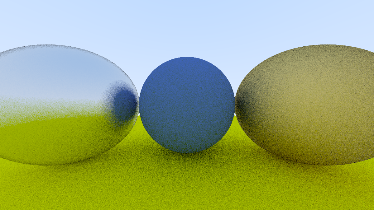
The world is built in the main function. This is actually one of my favorite parts of the system. Once objects (like Spheres) are defined, you can compose a world to your liking. Something I thought would be interesting would be to take this further and make a simple domain specific scripting language to compose the world programatically. The compiler’s backend format could just be a Python list that looks like the one in the main.
ray_tracer2/main.py
def main(output_image: str, image_width: int, anti_aliasing: int):
    world = World(
        hittable_list=[
            Sphere(center=[0.0, -100.5, -1.0], radius=100.0,
                   material=Lambertian(albedo=[0.8, 0.8, 0.0])),
            Sphere(center=[0.0, 0.0, -1.2], radius=0.5,
                   material=Lambertian(albedo=[0.1, 0.2, 0.5])),
            Sphere(center=[-1.0, 0.0, -1.0], radius=0.5,
                   material=Metal(albedo=[0.8, 0.8, 0.8], fuzz=0.3)),
            Sphere(center=[1.0, 0.0, -1.0], radius=0.5,
                   material=Metal(albedo=[0.8, 0.6, 0.2], fuzz=1.0)),
        ],
        tmin=0.001,
        tmax=1000000
    )
This was the first time I used the abstract class package in Python, abc. Taking an object-oriented approach certainly made the implementation more enjoyable, for example as I added new types of surface materials. Later in the book, there will be new types of hittables like rectangular prisms.
@dataclass
class Hittable(ABC):
    material: 'Material'

    @abstractmethod
    def hit(self, ray: Ray, tmin: float, tmax: float) -> (HitRecord, bool):
        return


@dataclass
class Sphere(Hittable):
    center: np.ndarray
    radius: float

    def hit(self, ray: Ray, tmin: float, tmax: float) -> (HitRecord, bool):
        ...
You may have also noticed I’m a fan of dataclasses. By decorating a class with @dataclass, it automatically generates implicit constructors with parameters to initialize member variables. It also reminds you to specify the type of your member variables.
Performance
The images started taking noticeably longer to generate, especially after adding anti-aliasing. So let’s profile the code.
Here are my CPU specs from lscpu:
  Model name:             11th Gen Intel(R) Core(TM) i5-1145G7 @ 2.60GHz
    CPU family:           6
    Model:                140
    Thread(s) per core:   2
    Core(s) per socket:   4
    Socket(s):            1
Let’s try generating a 400x225 image with 10 AA samples. Using Python’s cProfile package and running the program with only one process:
$ python3 -m cProfile -o cprofile.log ray-tracer2.py
And this python script to view the output:
import pstats
p = pstats.Stats('cprofile.log')
p.sort_stats('tottime').print_stats(50)
         132493209 function calls (131083200 primitive calls) in 181.877 seconds

   Ordered by: internal time
   List reduced from 1551 to 50 due to restriction <50>

   ncalls  tottime  percall  cumtime  percall filename:lineno(function)
  9225760   68.206    0.000   76.258    0.000 ray_tracer2/hittable.py:33(hit)
  1455329   17.573    0.000   37.015    0.000 ray_tracer2/utils.py:3(random_unit_vec)
    90000    9.651    0.000  181.106    0.002 ray_tracer2/camera.py:49(render_px)
  2872704    7.461    0.000   12.666    0.000 .venv/lib/python3.12/site-packages/numpy/linalg/_linalg.py:2566(norm)
  3673241    6.314    0.000    6.314    0.000 {method 'reduce' of 'numpy.ufunc' objects}
   900000    5.894    0.000   24.630    0.000 .venv/lib/python3.12/site-packages/numpy/lib/_arraypad_impl.py:545(pad)
   566264    5.216    0.000   22.605    0.000 ray_tracer2/material.py:21(scatter)
  3330462    4.644    0.000    4.644    0.000 ray_tracer2/ray.py:10(trace)
   851111    4.603    0.000    9.125    0.000 ray_tracer2/ray.py:13(colorize_miss)
  3673241    4.569    0.000   11.514    0.000 .venv/lib/python3.12/site-packages/numpy/_core/fromnumeric.py:69(_wrapreduction)
  2306440    4.390    0.000   80.648    0.000 ray_tracer2/hittable.py:86(hit)
2306509/900000    4.246    0.000  145.980    0.000 ray_tracer2/camera.py:32(ray_color)
   900000    4.102    0.000    5.799    0.000 .venv/lib/python3.12/site-packages/numpy/lib/_arraypad_impl.py:86(_pad_simple)
  1800000    3.730    0.000    7.646    0.000 .venv/lib/python3.12/site-packages/numpy/lib/_arraypad_impl.py:470(_as_pairs)
  3673241    3.542    0.000   15.732    0.000 .venv/lib/python3.12/site-packages/numpy/_core/fromnumeric.py:2255(sum)
   889065    3.251    0.000   29.325    0.000 ray_tracer2/material.py:38(scatter)
   900000    2.738    0.000    3.503    0.000 .venv/lib/python3.12/site-packages/numpy/lib/_arraypad_impl.py:129(_set_pad_area)
 30475039    2.532    0.000    2.532    0.000 .venv/lib/python3.12/site-packages/numpy/_core/multiarray.py:750(dot)
  2872705    2.343    0.000    2.343    0.000 {method 'dot' of 'numpy.ndarray' objects}
  4402304    2.102    0.000    2.102    0.000 {built-in method numpy.array}
  4672704    1.522    0.000    1.522    0.000 {method 'ravel' of 'numpy.ndarray' objects}
  4672704    1.107    0.000    1.107    0.000 {built-in method numpy.asarray}
   900000    0.772    0.000    0.772    0.000 .venv/lib/python3.12/site-packages/numpy/lib/_arraypad_impl.py:58(_view_roi)
  1800000    0.765    0.000    0.765    0.000 .venv/lib/python3.12/site-packages/numpy/lib/_arraypad_impl.py:33(_slice_at_axis)
  2872704    0.735    0.000    1.021    0.000 .venv/lib/python3.12/site-packages/numpy/linalg/_linalg.py:128(isComplexType)
  5745684    0.706    0.000    0.706    0.000 {built-in method builtins.issubclass}
  3808230    0.697    0.000    0.697    0.000 {built-in method math.sqrt}
  3689370    0.678    0.000    0.678    0.000 {built-in method builtins.isinstance}
   900000    0.649    0.000    1.457    0.000 .venv/lib/python3.12/site-packages/numpy/_core/fromnumeric.py:51(_wrapfunc)
  3673390    0.631    0.000    0.631    0.000 {method 'items' of 'dict' objects}
  1800000    0.627    0.000    0.627    0.000 .venv/lib/python3.12/site-packages/numpy/lib/_arraypad_impl.py:109(<genexpr>)
   900000    0.606    0.000    0.606    0.000 {method 'round' of 'numpy.ndarray' objects}
   900000    0.606    0.000    2.063    0.000 .venv/lib/python3.12/site-packages/numpy/_core/fromnumeric.py:3360(round)
   900001    0.538    0.000    0.538    0.000 {built-in method numpy.empty}
  1800000    0.531    0.000    0.531    0.000 .venv/lib/python3.12/site-packages/numpy/lib/_arraypad_impl.py:120(<genexpr>)
  3673241    0.480    0.000    0.480    0.000 .venv/lib/python3.12/site-packages/numpy/_core/fromnumeric.py:2250(_sum_dispatcher)
   900000    0.425    0.000    0.425    0.000 {method 'astype' of 'numpy.ndarray' objects}
  2355329    0.368    0.000    0.368    0.000 <string>:2(__init__)
  2872704    0.354    0.000    0.354    0.000 .venv/lib/python3.12/site-packages/numpy/linalg/_linalg.py:2562(_norm_dispatcher)
      2/1    0.289    0.145  181.985  181.985 ray_tracer2/camera.py:68(render)
...
That’s over 3 minutes for this tiny thing!
I sorted by tottime, the total time spent in the given function excluding time made in calls to sub-functions. This helps us isolate time spent in the business logic within a function’s scope. As expected, the compute-heavy hit() function is at the top of the list.
The random_unit_vec function is a (distant) second. This may be due to its iterative nature:
def random_unit_vec() -> np.ndarray:
    """
    Generate a random unit vector with (0,0) origin and |vec|=1.
    """
    sample = np.random.rand(3)*2 - 1
    ss = np.sum(np.square(sample))
    while (ss > 1) or (ss < 1e-160):
        sample = np.random.rand(3)*2 - 1
        ss = np.sum(np.square(sample))

    return sample/np.linalg.norm(sample)
We see np.linalg.norm near the top, which is used by hit().
2872704 7.461 0.000 12.666 0.000 .venv/lib/python3.12/site-packages/numpy/linalg/_linalg.py:2566(norm)
Adding multiprocessing to Python programs is a low-hanging fruit that I love to pick. Paired with tqdm, it provides a great way to speed up embarassingly parallel applications with a nice progress bar.
See commit b55d037 to see a simple example of how to do so.
Of course, this is not for free. The overhead of using multiprocessing even with only 1 process can be non-negligible. That’s why I added a bypass for single-process runs in commit 4660793.
By using 8 workers, the runtime reduces to less than 1 minute! This is still only a 3x improvement, which goes to show the overhead.
$ python3 -m cProfile -o cprofile.log ray-tracer2.py -p 8
...
         741496 function calls (735497 primitive calls) in 50.173 seconds